
Introduction
The Australian National Electricity Market (NEM), like many other international competitive market based electricity systems, must address system security and dispatch challenges associated with the introduction of increasing levels of intermittent generators. Both wind and solar power plants are being integrated into an existing market design that was based on the scheduled dispatch of hydro, coal and gas power plants. As countries respond to their agreed emission targets, intermittent generators are now a substantial proportion of the generation portfolio and the need to efficiently dispatch and manage system security is becoming critical in many international electricity markets.
As noted in [1], Wind Power Plants (WPP) in the NEM are currently dispatched as a semi-scheduled generator and can generate at any level unless constrained by network or pricing constraints. Dispatch intervals within the NEM are co-optimized between energy and Frequency Control Ancillary Services (FCAS) market bids with the NEM dispatch engine (NEMDE) optimizing the price paid by the market for both energy and ancillary services by analyzing the market offers, capability of all generating units, loads, and unit ramp rates.
For NEMDE to optimally dispatch a generator, the Australian Energy Market Operator (AEMO) requires accurate information on the prevailing conditions at the wind power plant. The existing AEMO Australian Wind Energy Forecasting System (AWEFS) uses a mixture of persistence forecasts, wind speed and turbine availability to create the Unconstrained Intermittent Generation Forecast (UIGF) for wind power plants to produce a central forecast ranging from 5 minutes to 7 days.
Changes in the past 12 months [2] have increased the amount of SCADA information sent to AEMO by wind power plants to augment the inputs to NEMDE, including an optional estimated power capability of the wind power plant: a signal from the SCADA system using vendor specific variants of a “capability right now” (also known as “Possible Power”, “Capable Power”, “Park Potential Power” or “Active Power Available”). The challenge with using a ‘now’ value is that the dispatch algorithm is working towards a power system security solution for 5 minutes into the future.
As NEM wind power plants progressively work towards implementing FCAS, the criticality of ensuring that the power system either a) takes account of the variability in the wind forecasts coming from the wind power plants in the coming 5-7 minutes and follows the wind direction, or b) sets an appropriate dispatch level to ensure wind variability is minimized [1], becomes even more important for market and power system operators.
Accurate 5 minute wind forecasts are critical for power system stability assessments which continually assess the power system to ensure adequate MW capability is available for contingency-based events. As WPP progressively provide ancillary services, power system operator confidence that the WPP will be able to provide the enabled contingency response will be paramount.
Forecasting approaches
There are many different wind forecasting techniques that have been used for predicting the output of wind power plants and the nature of the approaches used is determined by the forecasting horizons required and the time scales being studied. A detailed review of published wind power and speed forecasting techniques can be found in [3] and classifies the published forecasting approaches based on their intended time horizons and intended application.
Time-scale Classification for Forecasts [3]:
| Time horizon | Range | Applications |
|---|---|---|
| Very short-term | Few seconds to 30 minutes ahead | Electricity market clearing Regulation actions |
| Short-term | 30 minutes to 6 hours ahead | Economic load dispatch planning Load increment/decrement decisions |
| Medium-term | 6 hours to 1 day ahead | Generator online/offline decisions Operational security in day ahead markets Maintenance scheduling |
| Long-term | 1 day to 1 week or more ahead | Unit commitment decisions Reserve requirement decisions |
A more recent study [4] also includes a summary of the recent advances for wind forecasting and power prediction including global to local scales, ensemble forecasting and upscaling and downscaling processes.
Based upon the time scale of the forecasting required, the most common forecasting techniques developed and reported can be classified as follows.
Persistence Method
The “Naive Predictor” is used as the benchmark for many forecasting techniques and simply uses the wind speed or generation at time t as the forecast for a later time [5].

The equation specifies for the persistence forecast that the power forecast for time t + k made at the time origin t is the measured power at time t. Many papers have made the point that for very short to short time scales, the persistence forecast performs better than many forecasting techniques and is very difficult to improve upon [4][5].
Physical approach
Physical systems are based on modelling the physical atmosphere and environmental conditions of the wind power plant and often use weather services on a course grid adapted to the location and topology of the site. Complex mathematical models used by Numerical Weather Prediction (NWP) approaches are provided by weather services to produce forecasts based on temperature, pressure, surface conditions and roughness and are run a few times over a single day for timescales up to 7 days and are therefore only suited to medium to long time-scale forecasting.
Machine learning and statistical approaches
Modern machine learning techniques and the availability of cheap fast computing resources have presented the opportunity to significantly improve the forecasting capabilities of wind power plants and provide reliable short term forecasts that are a substantial improvement of the simple persistence forecasts that remain the benchmark for short time-scale generation forecasting techniques.
The forecasting of the short time-scale wind generation for the integration of wind power into the Australian NEM was described in the early stages of the market in a series of papers describing the modelling of Tasmanian wind power plants in advance of Tasmania being connected to the Australian mainland NEM market with the Basslink DC inter-connector using a combination approach of ANN models and fuzzy inference systems [6][7][8]. These papers correctly anticipated the requirement of the NEM to be able to accurately forecast wind power plants with the anticipated increased participation of renewable wind energy, the need for reliable dispatch of generators and the requirements for the provision of ancillary services.
Many short-term modelling approaches have been used for the wind generation forecasting problem. Wake effects and physical configuration of offshore wind power plants was presented in [9] where possible power forecasts were made using SCADA plant measurements and numerical wake models that focused on the interaction effects between turbines that are common to many wind power plants locations.
Other machine learning approaches for short term power forecasting have included Support Vector Machines [10], neural networks and adaptive Bayesian learning [11] and k-means clustering with ANN models [12]. The modelling approach in this paper is based on an initial experimentation process where a wide variety of machine learning approaches were evaluated, and an approach formulated that provided the best combination of predictive power and computational efficiency and performance to produce a robust and practical short time-scale wind power generation forecast for a wide variety of conditions. A standardized performance evaluation of short term wind power prediction models has been proposed by [5] and shall be used for the operational framework for the presented case study and the evaluation and comparison of the model results.
Given that the focus of this research is to find a reliable and effective forecasting approach over a single time horizon of 5 minutes, many of the lead time measures proposed in [5] are not appropriate for this study.
Evaluation and comparison of forecasting models
The main measure that will be used for the forecast model development, evaluations and comparisons will be based on the Root Mean Squared Error (RMSE) value defined as:

And for model evaluation, the Mean Absolute Error (MAE) shall also be used:

Statistically the MAE(k) is associated with the first moment of the prediction error that are directly related to the produced energy and the RMSE(k) values are associated with the second order moment relating to the variance of the prediction error. All error measures are calculated using the prediction error e(t + k|t).
For comparisons between models to highlight any relative improvement of one technique or set of parameters, a relative gain will be used to measure the improvement with respect to the reference model that will be the persistence model for all studies:

Here the EC is the Evaluation Criterion such as MAE or RMSE for the reference persistence model and for the forecasting model being considered.
Characteristics of the studied wind plant
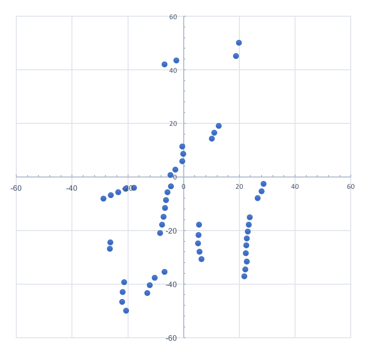
Figure 1: Normalized turbine layout of studied wind power plant
The studied wind power plant is a wind generator located in South East New South Wales, Australia with 51 turbines incorporating a mixture of Vestas V90 and V100 type 1.8 MW, 2 MW and 3 MW turbines. Total generation capacity for the wind power plant is 107 MW. The normalized turbine layout where the dominant axis has been mapped to a 100 unit nominal length is shown in Fig. 1.
The wind power plant uses the HARD software Infolite SCADA interface collecting very detailed data at a polling frequency of one minute, including a substantial range of turbine measurements and possible power estimate for the entire plant and was selected for the initial study to ensure a wide range of data could be considered.
The turbine locations for the wind power plant are a mix of hill-top, increasing gradient as well as flatter landscape profiles with a vertical distance between the lowest and highest wind turbines of nearly 90 m at approximately 960 m above sea level. The variation in site topology and turbine types presents challenging operating conditions and an even more challenging forecasting environment.
Forecasting approach
Early exploration and models
The initial investigation explored the nature of the very short-term forecasting problem from the perspective of using SCADA data that was easily available from common wind power plant control systems. Typically, the minimum data that is available from the control system are the meteorological measurements at key positions on the power plant site, individual turbine generation, turbine availability and total plant generation. Additionally, some power plants also measure wind speed and direction at the turbine nacelle, nacelle direction and calculate a possible power measurement for the current plant state.
The initial investigation of the short-term wind forecasting problem is discussed in detail in a previous paper [13] and this current paper shall focus only on the development of the turbine cluster and ensemble model and later developments and application of that model.
Turbine cluster & ensemble generation forecast model
Previous studies that used a turbine clustering approach for the short-term forecasting of wind power plant generation used unsupervised statistical techniques such as k-means clustering that groups a set of observations around observed initial cluster centres [12] and supervised learning techniques, such as the k-nearest neighbors technique, that was considered in the initial exploratory investigation.
The turbine clustering approach used for this study considers the static locations of the turbines, the local topology and the dynamic environmental conditions. Each of the turbines are assigned to a static cluster for a set of conditions and then an overall ensemble model is then used by aggregating the predicted generation cluster forecasts to produce a forecast for the entire wind power plant.
For this study, stochastic gradient boosting (SGB) models [14] were used for the individual cluster models and both stochastic gradient boosting and ANN models were used for the ensemble models, thus producing a forecast for the entire wind power plant over a very large range of differing input environmental conditions.
Turbine ensemble deep learning model
Although the initial results for the turbine cluster and ensemble model were encouraging for the studied wind power plant, application of the same technique to other generators did not reproduce the performance of the forecasting model with small improvements in RMSE and MAE in comparison to the persistence model for one plant and, for another, virtually no improvement from the persistence model at all. The reasons for the lack of generalization of the model and poor performance when applied to these other wind power plants is not yet fully understood at this stage, but there were varying sector management policies and network support functions present that may need to be identified and excluded or nullified prior to training the model before reasonable results can be produced.
A more general alternative ensemble approach without fine grained clustering was then formulated to attempt to improve the performance of the forecasting model and to understand if there was a fundamental issue with the data or plant environment that would prevent a reasonable forecasting model from predicting short-term generation.
A new set of data was produced using a single ensemble of model data for the same range of dynamic environmental conditions and that data was then normalized for use with a deep learning ANN model. The data included individual turbine generation, change in generation, “one-hot” encoding of availability and a range of summary statistics of MET data producing about 133 input variables.
To determine the influence of the forecasting approach on the wind power forecasting model, the same ensemble data was also used to train a Stochastic Gradient Boosting machine learning model for comparison to the ANN model.
Forecasting results
Turbine cluster & ensemble forecast results
Clustering the turbines into groups and running ensemble models to produce the power plant forecast had a very substantial effect on the model training times and computational resources required to train the model. For all the initial investigation and the single generator machine learning models it was feasible to train and run the evaluations on a single MacBook Pro laptop but the learning times for the clustered model took too long to complete for this approach to be feasible for the clustered models.
A Compute Optimized 32 core 60 GB memory AWS C3.8xlarge instance running Ubuntu 16.04 was used to develop the clustering and ensemble turbine models where typical run times for each training and evaluation run for a turbine cluster model were about 24 hours on this optimized AWS instance.
Once the model has been trained and developed, evaluation is a very quick operation making both the stochastic gradient boost and ANN models ideally suited for production deployment.
For the cluster model, 314,357 observations were used with the input data being randomly split into 90% of the data forming the training set with 285,779 observations and an independent validation data set comprising 28578 records. No part of the validation set was used in the training of the turbine cluster or ensemble model. The procedure for the training of the model is shown in Fig. 2 where the validation dataset has not been used in any part of the training of the model.
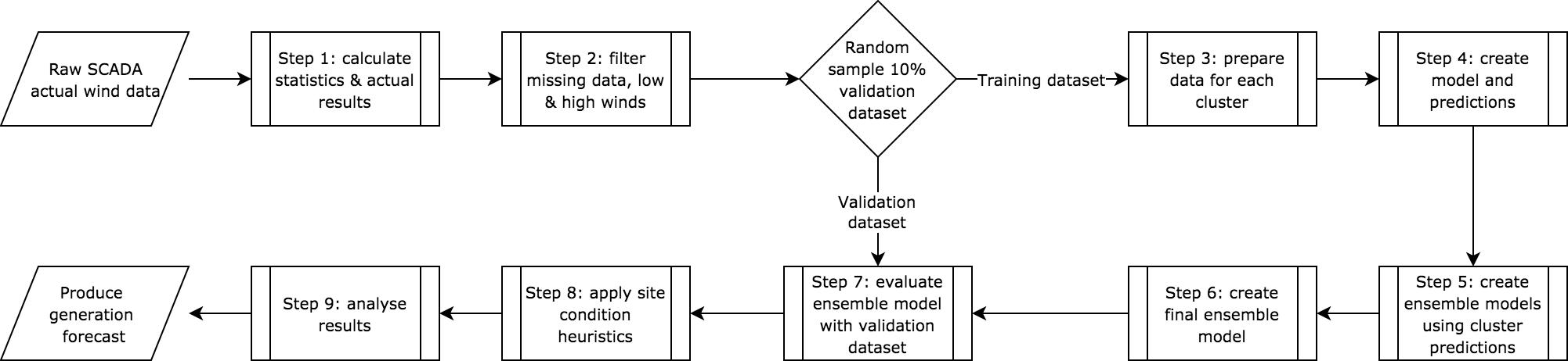
Figure 2: Procedure for developing the short-term generation model (click imageto view in more detail)
A k-fold cross-validation approach was used to train the models with 10 splits on the training data and a negative mean squared loss function was used for the model training.
Various combinations of input fields were used for the stochastic gradient boosting model for both the individual turbine clusters and the ensemble model. The SGB model can display the feature importance of each of the input fields and so by determining the contribution each field makes to the forecast results; the models can be refined.
There are many different parameters that are available to be tuned for the SGB model such as the learning rate, depth of trees, number of trees and the minimum child weight and the results were relatively insensitive to most parameter changes and continued to find consistent optimal values even when large ranges of parameters were tested. The number of trees parameter was the exception where large numbers of trees would give low training evaluation scores but perform worse on the independent validation dataset indicating that the model was over-fitted to the training data.
The turbine cluster and ensemble model using the SGB model for both the clusters and the ensemble produced a range of RMSE improvements in comparison to the persistence forecast for this preliminary model of 7.2% to 10.7% and for the MAE 9.1% to 10.4%. Considering the early stages of development of the forecasting model and the recent completion of the clustering implementation, the observed results are very encouraging and certainly much better than any of the single generation forecast wind power plant models.
Lastly an ANN ensemble model was run on the ensemble data using the SGB model for the turbine clusters without any refinement or development just prior to this paper being completed with resulting improvements in RMSE compared to the persistence forecast of 8.8% and MAE of 7.5%. Given that no tuning or development of the ANN model has been possible, it may prove that ANN is a more effective means of producing the final ensemble forecast rather than the stochastic gradient model and this result influenced the decision to develop the later ensemble deep learning model.
Turbine ensemble deep learning model results
The turbine ensemble deep learning forecasting models were trained using the same training dataset for the previous cluster and ensemble model.
A wide variety of ANN topologies were tested using the deep learning Theano library, incorporating wide and deep networks and various formulations of hidden layers, using 20% of the training data as validation during the supervised training process. The final trained model was then evaluated on the independent validation data set and compared to the equivalent persistence model error results on the same validation data to determine if any improvement had been produced. The best model results produced using the ANN machine learning model was an improvement in RMSE of 11.9% and for the MAE of 11.4% in comparison to the persistence forecast and therefore produced better results than the turbine cluster and ensemble model.
Fig 3. shows the error distribution by wind direction for the modelled wind power plant of the filtered SCADA data with the equivalent distributions of persistent RMSE, model RMSE and the improvement in RMSE between the naïve persistent model and the best ANN model. The top chart in Fig. 3 shows the wind direction distribution of the number of observations, the next chart the RMSE persistent errors, then the forecast RMSE errors and lastly the bottom chart shows the improvement of the RMSE of the forecast model in comparison to the persistence model.
The same turbine ensemble data formulation was then used to train a Stochastic Gradient Boosting machine learning model with a variety of learning parameters and produced a substantial improvement in the RMSE of 14.2% and MAE of 14.6% and has demonstrated the best forecasting performance of any of the machine learning models currently being developed.
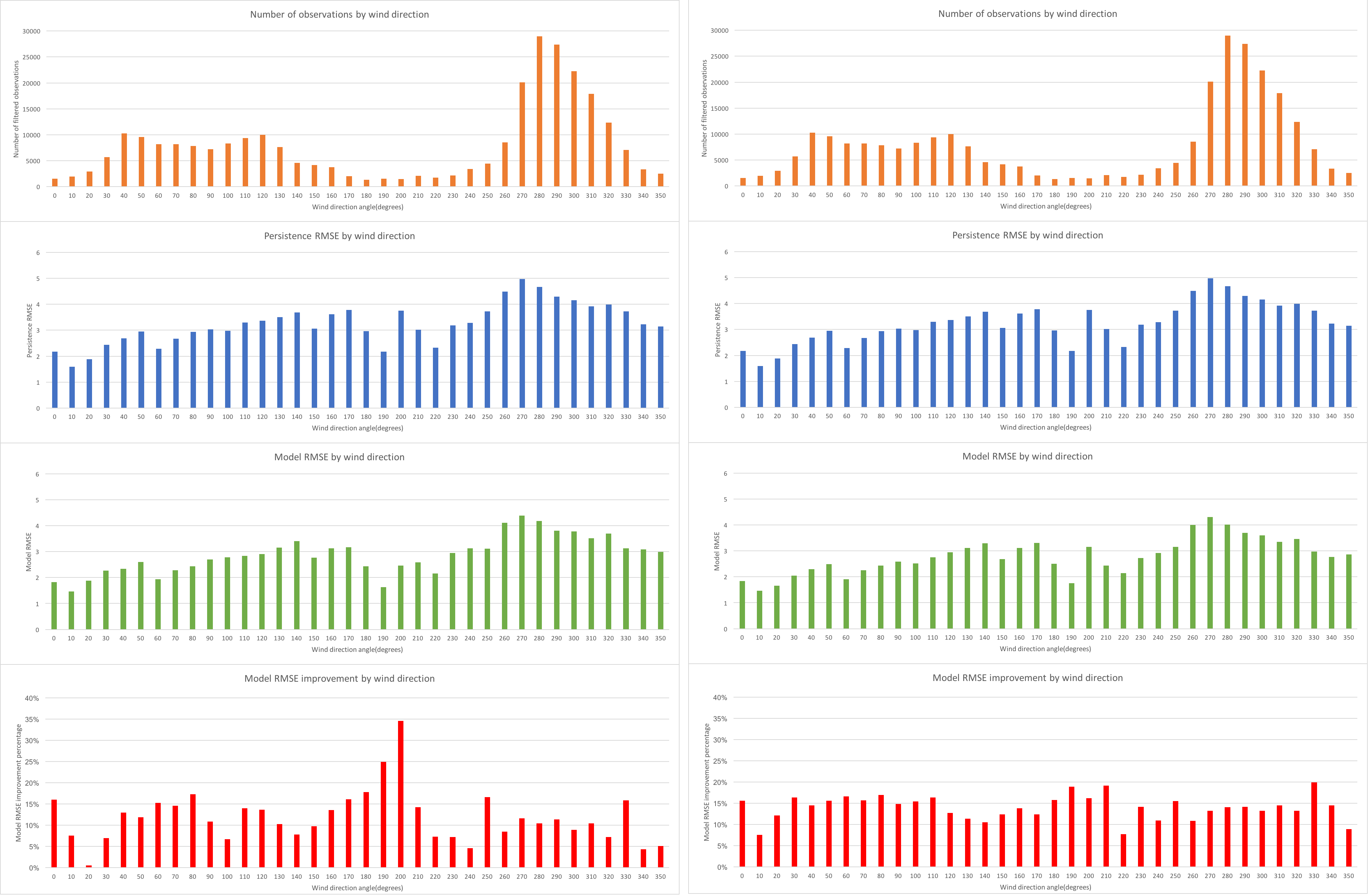
| Figure 3: ANN model RMSE error distribution by wind direction | Figure 4: SGB model RMSE error distribution by wind direction |
Fig 4. shows the wind direction distribution of the RMSE errors and improvement in RMSE with respect to the persistence model RMSE errors by wind direction and it can be seen by comparison to the ANN results shown in Fig 3. using the same chart format, that the SGB model improvements are much more evenly spread across all the wind directions, but the ANN model produced substantially better performance on a small number of wind directions.
By selectively using the ANN model and SGB model based on measured wind direction, a hybrid model improvement in RMSE of 15.0% and MAE of 14.6% was achieved but how practical combining the models is for production forecasting implementations remains to be demonstrated. These results are very encouraging, and the authors have been unable to find any reported instances of better wind forecasting error rates in comparison to persistence forecasts for very short term wind generation.
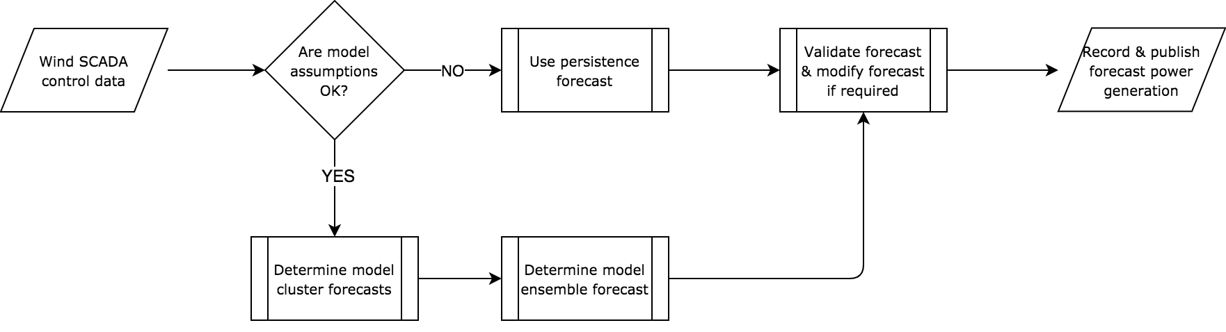
Figure 5: Procedure for producing generation forecasts (click image to view in more detail)
The current study has been undertaken with the ultimate objective of implementing the developed and refined forecasting model into a production device that can be implemented within the wind power plant SCADA system.
The production forecast implementation is required to operate under a wide range of input conditions and must be robust and reliable. If the inputs to the forecast model do not meet the model validation requirements, the forecast model will revert to using the persistent forecast value rather than risk the production of an erronous forecast value and produce poor outcomes (Fig. 5).
Individual wind power plant locations, site details and production data will be used to create a dedicated set of models for the generator. Once a suitably trained set of models has been developed for a specific site, the implementation of the new forecasting technique will be directed toward replacing the existing Australian NEM intermittent generator AWEFS dispatch forecast with the revised, trained estimation of the likely generation in the coming 5 to 7 minute dispatch period.
The implementation of the forecasting device will have the following effects for both the generator and the system operator:
Provide a more accurate forecast for the wind power plant to reduce its deviation from the dispatch target calculated by AEMO and thereby reducing any ‘causer-pays’ penalties [15];
allow the wind generator to potentially participate in raise FCAS contingency and regulation markets by providing accurate, unconstrained generation forecasts; and
contributing to the reduction in the uncertainty of individual wind generators, provide more accurate regulation requirement estimations for AEMO to ensure appropriate control of secondary-order primary frequency control.
The device is being designed as a dedicated server that will have a direct connection to the SCADA system through the modbus, DNP3 or possibly IEC 61400-25 protocols and can provide a web service interface, write directly to the SCADA and database for later validation and analysis. The device will be supported remotely and will be updated at regular intervals with model updates and refinements.
Conclusions and future work
This paper presents the encouraging preliminary results of the development of a dedicated machine learning device for the 5 to 7 minute forecasting of generation for wind power plants. Further development of the model is required to improve the clustering, tune the machine learning algorithms and demonstrate the capabilities and robustness of the forecasting approach over a sustained period of operation and for a larger set of diverse wind power plants.
Acknowledgment
The authors would like to thank Pacific Hydro Australia for permission to publish the forecasting results for their wind power plant. Also, this research would not be possible without the availability of the many excellent open source projects such Python, Pandas, Scikit-Learn, Keras, Theano, NumPy and Weka, that were used in this study.
References
[1] Jennings, R., Dyson, J. and Summers, K., 2016, November. The maturing of wind integration in Australia: Improvements required in market operation for more consistent, economic and efficient dispatch outcomes. 15th Wind Integration Forum, Vienna.
[2] http://www.aemo.com.au/Stakeholder Consultation/Consultations/ AWEFS and ASEFS Stakeholder Consultation, accessed 27 July 2017.
[3] Soman, S.S., Zareipour, H., Malik, O. and Mandal, P., 2010, September. A review of wind power and wind speed forecasting methods with different time horizons. In North American Power Symposium (NAPS), 2010 (pp. 1-8). IEEE.
[4] Foley, A.M., Leahy, P.G., Marvuglia, A. and McKeogh, E.J., 2012. Current methods and advances in forecasting of wind power generation. Renewable Energy, 37(1), pp.1-8.
[5] Madsen, H., Pinson, P., Kariniotakis, G., Nielsen, H.A. and Nielsen, T.S., 2005. Standardizing the performance evaluation of short-term wind power prediction models. Wind Engineering, 29(6), pp.475-489.
[6] Potter, C., Ringrose, M. and Negnevitsky, M., 2004, September. Short-term wind forecasting techniques for power generation. In Australasian Universities Power Engineering Conference (AUPEC 2004) (pp. 26-29).
[7] Potter, C.W. and Negnevitsky, M., 2006. Very short-term wind forecasting for Tasmanian power generation. IEEE Transactions on Power Systems, 21(2), pp.965-972.
[8] Negnevitsky, M., Johnson, P.L. and Santoso, S., 2007. Short term wind power forecasting using hybrid intelligent systems.
[9] Gocmen, T., Giebel, G., Rethore, P.E. and Leon, J.P.M., 2016, November. Uncertainty quantification of the real-time reserves for offshore wind power plants. 15th Wind Integration Forum, Vienna.
[10] Zhou, J., Shi, J. and Li, G., 2011. Fine tuning support vector machines for short-term wind speed forecasting. Energy Conversion and Management, 52(4), pp.1990-1998.
[11] Blonbou, R., 2011. Very short-term wind power forecasting with neural networks and adaptive Bayesian learning. Renewable Energy, 36(3), pp.1118-1124.
[12] Kusiak, A. and Li, W., 2010. Short-term prediction of wind power with a clustering approach. Renewable Energy, 35(10), pp.2362-2369.
[13] Mackenzie, H.J., and Dyson, J., 2017, Short-Term Forecasting of Wind Power Plant Generation for System Stability and Provision of Ancillary Services, 1st International Conference on Large Scale Integration of Renewable Energy in India, New Delhi.
[14] Friedman, J.H., 2002. Stochastic gradient boosting. Computational Statistics & Data Analysis, 38(4), pp.367-378.
[15] Operations Department – Systems Performance & Commercial, Causer Pays Procedure: Determination Of Contribution Factors For Regulation FCAS Cost Recovery, AEMO, 2017.
About our Guest Author
|
|
Dr. Harley Mackenzie Mackenzie is the Managing Director of HARD software that has been operating in the energy industry for nearly 20 years after having worked with Yallourn Energy and completing his Phd on modelling combustion processes. He is also a director of a new venture Dispatch Solutions with Jonathon Dyson looking at short term forecasting for solar and wind farms and providing independent trading and operations services.
HARD Software develops technical tools and solutions for trading, generation and retail operations in the Australian NEM and International energy markets as well as providing consulting services in energy, risk management and aviation. His current passions are focussed on reducing the costs of FCAS services for intermittent generators, providing effective wind and solar software tools and developing short term wind and solar forecasting solutions. Email: hjm@hardsoftware.com You can find Harley on LinkedIn here. |

Right exactly. That”s why it”s *NOT* Internet of Things. It”s just Connected Things On A Private Network. We used to do that with leased lines and AX.25. Big wup. Thanks for re-inventing SCADA. You are still tied to a single wireless technology, to a single MVNO, to using SIM cards, and your devices only talk to the cloud, not to each other.